机器学习

Machine Learning

The Definition

an older one:

the field of study that gives computers the ability to learn without being explicitly programmed ——Arthur Samuel

an modern one:

A computer program is said to learn from experience E with respect to some class of tasks T and performance measure P, if its performance at tasks in T, as measured by P, improves with experience E ——Tom Mitchell

Example: playing checkers.

• E = the experience of playing many games of checkers

• T = the task of playing checkers.

• P = the probability that the program will win the next game.

So, the machine learning is said to through the task, get the experience, finally learn to achieve the ideal goal (solve some problem)

Supervised learning

We give out a “right answer”,(more like a test data set) Then the task is to generate more data that are similar to the “right answer”

In supervised learning, we are given a data set and already know what our correct output should look like, having the idea that there is a relationship between the input and the output.

categories:

• regression

  continuous output

• classification

  discrete output

Unsupervised learning

In Unsupervised Learning, we have the same data set, but we have no idea what exactly the task is and what to do next. It seems different since there is no such concept like attribute or tag(which means all the data is the same, there is no difference)

Unsupervised learning allows us to approach problems with little or no idea what our results should look like. We can derive structure from data where we don’t necessarily know the effect of the variables.

Example:

比如说今日头条上的所有新闻，它们虽然是根据一些专题进行分类，但是最开始都是一堆差不多的新闻数据。字节跳动内容算法将这些差不多的类似的新闻数据进行学习，最终得到了每个分类，但是并没有人指明这些类别应该按照什么标准进行划分，只是需要划分出来(automatically)。

Most of time, the usual method is cluster algorithm. Run that Alforithm, get the clustered result. (We never know the standard)

Cost Function

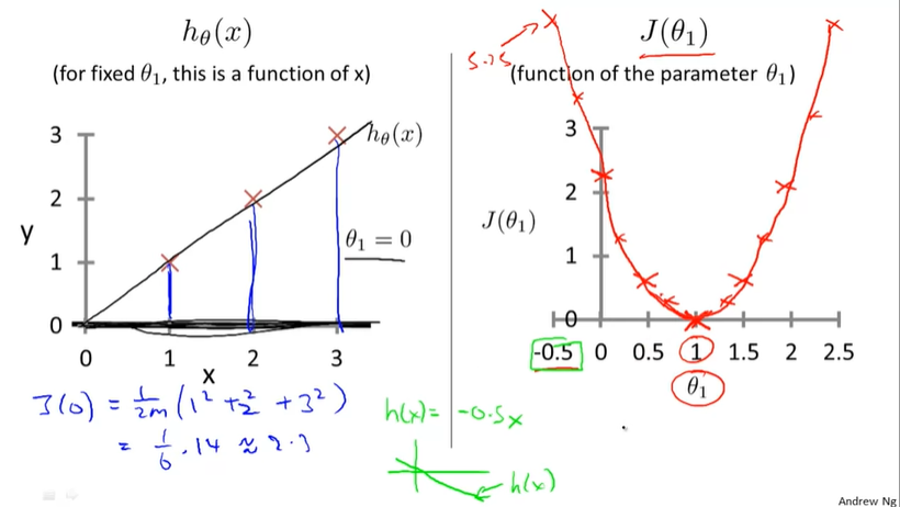
cost function is the same meaning of loss function(损失函数), the cost function(or loss funciton) can be descibed as $L(Y, f(X)) = (Y - f(X))^2$,(compare the result L with fact value Y) this means the less the value of cost function, the better the model fits.

the regular form of cost function:

$$J(\theta) = \frac{1}{2m}\sum_{i=1}^{m}(h_\theta(x^{(i)}) - y^{(i)})^2$$

所以你可以简单的理解成，J（代价函数）是一个根据$H_\theta$（假设函数）得到来的这个假设函数和现实的拟合程度，J越小，取这个$\theta$的值的时候拟合程度最好。

Hypothesis Function

对于Cost Function, 我们还是需要简单讲一下hypothesis function(假设函数)的，因为有了一个Hypothesis function, thus the cost function has its own meaning.

Hypothesis: $h_\theta = \theta_0 + \theta_1x$

Parameter: $\theta_0, \theta_1$

Cost Function: $J(\theta0,\theta_1) = \frac{1}{2m}\sum{i=1}^{m}(h_\theta(x^{(i)}) - y^{(i)})^2$

Goal: $mininmize J(\theta)$

Gradient Descent

当我们画出J的图像的时候，我们很想方便快捷的得出J值最小的时候，就需要有一个算法得到J最小的时候，这样我们就可以反推$\theta_0, \theta_1$，最终完成Hypothesis function的求出。

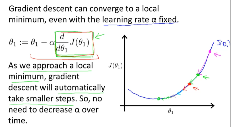
采用梯度下降的方法，就是将现在的观察点最为基点找到局部的最低点（在一个局部面积范围内），然后下降（Descent）之后找到另一个基点，以此类推找到最终的最低点（Global）。个人认为属于一种贪心算法。

The size of each step is determined by the parameter α, which is called the learning rate.

For example, the distance between each ‘star’ in the graph above represents a step determined by our parameter α. A smaller α would result in a smaller step and a larger α results in a larger step.

The gradient descent algorithm is:

repeat until convergence:

$$\theta_j := \theta_j - \alpha \frac{\delta}{\delta\theta_j} J(\theta_0, \theta_1)$$

Go Further

the α is also called as learning rate, it controls how much step we update that parameter $\theta_j$.

当然我们也知道对应的$\thetaj$是根据导数的值来改变的，也就是说，但我们越来越接近局部最优解（local optima）的时候，我们的step自动就会越来越小，因为倒数是越来越小（对应斜率）的。这意味着我们越接近最优解，我们迈的步子就越小（很符合收敛的概念_）

但是用这种写法就意味着我们最终只能得到局部最优（全局待解）

$$\theta_0 := \theta_0 - \alpha \frac{1}{m} \sum_{i=1}^m(h_\theta(x_i) - y_i) \\ \theta_1 := \theta_1 - \alpha \frac{1}{m} \sum_{i=1}^m((h_\theta(x_i) - y_i)x_i)$$

不过，当我们的cost function是一个凸函数的时候，我们找到的必然就是全局最优解了。

Linear Algebra Review

线性代数在这里都需要单独复习了，可想而知，对于整个Machine learning来说，线性代数是有多么重要了。

Vector

vector（向量）：表示一个只有一个一列的矩阵

即所有的矩阵元素都可以用$a_{1n}$来表示

但是你可能会疑惑，为什么是一列呢？我们在标准的线性代数的课程中学习到的实际上是一行的矩阵也能表示一个向量，此刻且先记住这个概念：一列的结果是为了将向量放到第二个乘数的位置，这样就可以得到一个矩阵的预测结果了。可以这么理解：

$$DataSet \times Hypothesis = Prediction$$

Multiplication

矩阵乘法也没有什么好说的，主要是对于结果来说，行数决定于前一个矩阵，列数决定于后一个矩阵。

可以这么理解：Matrix和Vector的乘法是得到一个预测结果，但是Matrix和Matrix（Vectors）相乘就是得到多个结果并进行比较。

Matrix Inverse

if A is an $m \times m$ matrix, it is also called an square

学过线性代数都知道，一个矩阵的逆（也就是逆矩阵）和乘原矩阵就得到单位矩阵（Identity Matrix）：

$$A^{-1} \times A = I$$

使用python求矩阵的逆（numpy）

import numpy as np
a=np.array([[1,2,3],[4,5,6],[7,8,9]]) # 初始化一个非奇异矩阵(数组)
print(np.linalg.inv(a))  # 对应于MATLAB中 inv() 函数

# 当然，矩阵对象可以通过 .I 更方便的求逆
A = np.matrix(a)
print(A.I)

Matrix Transpose

即矩阵的转置的概念，the sign is like this: $A^T$ and $A$

so obviously, $A^T_{ij} = A_ji$

Multiple Variables(Features)

simplify the fomula

$$h_\theta(x) = \theta_0 + \theta_1 x_1 + \theta_2 x_2 + ... + \theta_n x_n$$

for convenience of notation, define $x_0 = 1$.

then we have

$$x = \left(\begin{array}{c} x_0 \\ x_1 \\ x_2 \\ ... \\ x_n \end{array} \right) \qquad \theta = \left(\begin{array}{c} \theta_0 \\ \theta_1 \\ \theta_2 \\ ... \\ \theta_n \end{array} \right)$$

the $h_\theta(x)$ then can be transformed into:

$$h_\theta(x) = \theta^T x$$

Feature Scaling

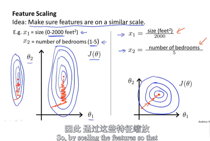
当一个变量$x_1$的影响要远大于$x_2$的情况下，J（cost function）的图像可能非常的窄，这样就相当于我们需要大量的时间和实践来完成全局最优解的求解。此时我们部分通过缩放变量来达到变量之间影响的均衡，这就是特征缩放（Feature Scaling）。

Usually, the range of the variable is regular to be scaled into [-1, 1], which means you shouldn’t put the range up to 100 or down to 0.0001(for example).

所以这就相当于是一种公式（而不是数据的）的预处理，当我们我们的变量的范围千差万别的时候，我们可以通过这种方式来使得变量变得范围差不多。

debug and choose α

if α is too small: slow convergence.

if α is too large: $J(\theta)$ may not decrease on every iteration; or may not converge.

to choose α, try
…, 0.001, 0.003, 0.01, 0.03, 0.1, 0.3, 1, …

Regulation

name	mean
m	the number of train sample
x	feature variable
y	output variable
:=	赋值语句
n	number of features
$x^{(i)}$	input(features) of $i^{th}$ training example(a vector)
$x^{(i)}_j$	value of feature j in $i^{th}$ training example